TensorFlow (5-2) Use Simple RNN to classify MNIST Images

This program comes from Ref[1] which demonstrates how to classify MNIST images with a simple RNN.

We modify the program in Ref[1] and break it in to pieces to discuss the core concept of RNN.

1. Define the parameters and summarize the variables:

#!/usr/bin/python3
import tensorflow as tf
from tensorflow.examples.tutorials.mnist import input_data

def variable_summaries(var):
    with tf.name_scope('summaries'):
        mean = tf.reduce_mean(var)
        tf.summary.scalar('mean', mean)
        with tf.name_scope('stddev'):
            stddev = tf.sqrt(tf.reduce_mean(tf.square(var - mean)))
        tf.summary.scalar('stddev', stddev)
        tf.summary.scalar('max', tf.reduce_max(var))
        tf.summary.scalar('min', tf.reduce_min(var))
        tf.summary.histogram('histogram', var)

# Define data dir and log dir
LOG_DIR = "logs/RNN_with_summaries"
mnist = input_data.read_data_sets("data/", one_hot=True)

# Define some parameters
element_size = 28
time_steps = 28
num_classes = 10
batch_size = 130
hidden_layer_size = 128

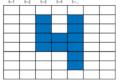
The MNIST image is viewed as a sequence of the vectors.

In this case, each column of the image is treated as a time_step and the element_size is the dimension of each vector in our sequence.

2. Define computational process of Vanilla RNN:

Recall the equation of the Vanilla RNN:

$$h_{t} = tanh(W_{x}x_{t}+W_{h}h_{t-1}+b)$$

#
# Vanilla RNN
#
_inputs = tf.placeholder(tf.float32, 
                         shape=[None, time_steps, element_size],
                         name='inputs')
y = tf.placeholder(tf.float32, 
                   shape=[None, num_classes],
                   name='labels')

with tf.name_scope('rnn_weights'):
    with tf.name_scope("W_x"):
        Wx = tf.Variable(tf.zeros([element_size, hidden_layer_size]))
        variable_summaries(Wx)
    with tf.name_scope("W_h"):
        Wh = tf.Variable(tf.zeros([hidden_layer_size, hidden_layer_size]))
        variable_summaries(Wh)
    with tf.name_scope("Bias"):
        b_rnn = tf.Variable(tf.zeros([hidden_layer_size]))
        variable_summaries(b_rnn)

def rnn_step(previous_hidden_state,x):
    current_hidden_state = tf.tanh(
                                tf.matmul(previous_hidden_state, Wh) +
                                tf.matmul(x, Wx) + b_rnn)
    return current_hidden_state

# Transpose the input before tf.scan()
# Input shape: (batch_size, time_steps, element_size)
# Output shape: (time_steps, batch_size, element_size)
processed_input = tf.transpose(_inputs, perm=[1, 0, 2])

initial_hidden = tf.zeros([batch_size,hidden_layer_size])

# Create a unrolled chain
all_hidden_states = tf.scan(rnn_step,
                            processed_input,
                            initializer=initial_hidden,
                            name='states')

tf.scan() returns a list of the state vectors. Because tf.scan() processes the input sequentially, the first dimension of the input is transposed to the dimension of time_steps.

3. Define the linear layer:

# Linear layer
with tf.name_scope('linear_layer_weights') as scope:
    with tf.name_scope("W_linear"):
        Wl = tf.Variable(tf.truncated_normal([hidden_layer_size, num_classes],
                                mean=0,stddev=.01))
        variable_summaries(Wl)

    with tf.name_scope("Bias_linear"):
        bl = tf.Variable(tf.truncated_normal([num_classes],
                                mean=0,stddev=.01))
        variable_summaries(bl)

#[start-cooperbear-mod]#
# def get_linear_layer(hidden_state):
#     return tf.matmul(hidden_state, Wl) + bl
#[end-cooperbear-mod]#

with tf.name_scope('linear_layer_outputs') as scope:
#[start-cooperbear-mod]#
    # # Iterate across time, apply linear layer to all RNN outputs
    # all_outputs = tf.map_fn(get_linear_layer, all_hidden_states)
    # # Get last output
    # output = all_outputs[-1]

    last_state = all_hidden_states[-1]
    output = tf.matmul(last_state, Wl) + bl
#[end-cooperbear-mod]#
    tf.summary.histogram('outputs', output)

with tf.name_scope('cross_entropy'):
    cross_entropy = tf.reduce_mean(
                           tf.nn.softmax_cross_entropy_with_logits_v2(logits=output, labels=y))
    tf.summary.scalar('cross_entropy', cross_entropy)

The image is read column by column.

Each column is passed to the neural network and return a state vector. The state vector is relative to the temporal result of the classification. Most important of all, the final state vector is relative to the result of the whole sequence.

The state vector is transformed to the classification result through the linear layer.

4. Select an optimizer and start trainning:

#
# Define optimizer and accuracy 
#
with tf.name_scope('train'):
    # Using RMSPropOptimizer
    train_step = (tf.train.RMSPropOptimizer(0.001, 0.9).
                    minimize(cross_entropy))

with tf.name_scope('accuracy'):
    correct_prediction = (tf.equal(
                                tf.argmax(y,1), 
                                tf.argmax(output,1)))
    accuracy = (tf.reduce_mean(
                    tf.cast(correct_prediction, tf.float32)))*100
    tf.summary.scalar('accuracy', accuracy)
merged = tf.summary.merge_all()


# Get a small test set
test_data = mnist.test.images[:batch_size].reshape((-1, time_steps, element_size))
test_label = mnist.test.labels[:batch_size]

# Train
#[start-cooperbear-add]#
from time import time
start = time()
#[end-cooperbear-add]#
with tf.Session() as sess:
    train_writer = tf.summary.FileWriter(LOG_DIR + '/train',
                                         graph=tf.get_default_graph())
    test_writer = tf.summary.FileWriter(LOG_DIR + '/test',
                                        graph=tf.get_default_graph())

    sess.run(tf.global_variables_initializer())
    for i in range(5000):
        batch_x, batch_y = mnist.train.next_batch(batch_size)
        batch_x = batch_x.reshape((batch_size, time_steps, element_size))
        summary,_ = sess.run([merged,train_step],
        feed_dict={_inputs:batch_x, y:batch_y})
        train_writer.add_summary(summary, i)

        if i % 1000 == 0:
            acc,loss, = sess.run([accuracy,cross_entropy],
                                 feed_dict={_inputs: batch_x, y: batch_y})
        
        print ("Iter " + str(i) + ", Minibatch Loss= " + \
               "{:.6f}".format(loss) + ", Training Accuracy= " + \
               "{:.5f}".format(acc))

        if i % 10:
            summary, acc = sess.run([merged, accuracy],
                                    feed_dict={_inputs: test_data, y: test_label})
            test_writer.add_summary(summary, i)
        test_acc = sess.run(accuracy, feed_dict={_inputs: test_data, y: test_label})
        print ("Test Accuracy:", test_acc)

#[start-cooperbear-add]#
end = time()
print("process time:", end-start)
#[end-cooperbear-add]#

Reference

[1] Tom Hope, Yehezkel S. Resheff, and Itay Lieder, Learning TensorFlow A Guide to Building Deep Learning Systems , O'Reilly Media (2017)

[2] Nikhil Buduma, Fundamentals of Deep Learning Designing Next-Generation Machine Intelligence Algorithms, O'Reilly Media (2017)

[3] Aurélien Géron, Hands-On Machine Learning with Scikit-Learn and TensorFlow Concepts, Tools, and Techniques to Build Intelligent Systems , O'Reilly Media (2017)